Equilibrium and Elasticity

Equilibrium and Elasticity

$Learning Objectives$

Define and apply the conditions for static equilibrium.
Calculate the center of mass and understand its relation to the center of gravity.
Define stress, strain, and understand their relationship through Hooke's Law.
Analyze material deformation including tension, compression, shear, and bulk stress.
Interpret proportional, elastic, yield, plastic, ultimate, and fracture landmarks without conflating them.
Calculate free thermal strain and fully restrained thermal stress for the stated linear-elastic model.

For a structure like a bridge or a building to serve its purpose, it must remain stationary and maintain its shape under various loads. This requires the principles of static equilibrium and an understanding of how materials deform (elasticity).

Static Equilibrium

$Static Equilibrium Concepts$

An object is in static equilibrium if it is completely at rest in our chosen frame of reference. This means it has no linear acceleration and no angular acceleration.

For a rigid body (an object whose size and shape do not change under load), two conditions must be met simultaneously for it to be in equilibrium.

Translational Equilibrium Condition

The vector sum of all external forces must be zero.

\Sigma \vec{F} = 0

Variables

Symbol	Description	Unit
$\Sigma \vec{F}$	Net external force	N

$Translational Equilibrium in 2D$

In 2D (xy-plane), the translational equilibrium condition breaks down into two scalar equations: $\Sigma F_x = 0$ and $\Sigma F_y = 0$ .

Rotational Equilibrium Condition

The vector sum of all external torques about any axis must be zero.

\Sigma \vec{\tau} = 0

Variables

Symbol	Description	Unit
$\Sigma \vec{\tau}$	Net external torque	$N\cdot m$

$Choosing an Axis of Rotation$

When applying the torque equation ( $\Sigma \tau = 0$ ), you are free to choose the axis of rotation anywhere you like. A strategic choice of axis (e.g., placing it exactly where an unknown force acts) will eliminate that unknown force from your torque equation, simplifying the math significantly.

$Interactive Simulation$

Use this torque balance model to see how lever arms and loads must offset each other for rotational equilibrium.

✓ Equilibrium

Left Load — CCW

20 kg

-3.0 m

Right Load — CW

30 kg

2.0 m

Moment Balance about O

\Sigma\tau_O = 588.6\,\mathrm{N\cdot m} - 588.6\,\mathrm{N\cdot m} = 0.0\,\mathrm{N\cdot m}

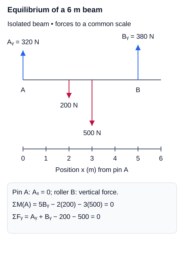
Rotational equilibrium: $\sum \tau_O = 0$ . The uniform beam weight passes through the pivot, so it contributes no moment about $O$ , but it is still included in the vertical reaction.

CCW Torque

588.60 N·m

CW Torque

588.60 N·m

Vertical Reaction R_y

588.60 N

Net Torque

0.00 N·m

Beam free-body diagram with two support reactions, a point load, and self-weight at its center — Static Equilibrium Requires a Complete FBD
Force equilibrium and moment equilibrium must be applied to the same isolated body with all external forces and lever arms shown.

Center of Gravity (CG)

$Center of Gravity (CG) Concepts$

The center of gravity is the point at which the entire weight of an object can be considered to act for the purpose of calculating torques due to gravity.

For a uniform object in a uniform gravitational field (like near the Earth's surface), the center of gravity coincides perfectly with the geometric center of mass (CM).

$x_{cm}$

The geometric center of a mass distribution.

Center of Mass for Discrete Masses

Calculates center of mass position for a system of discrete particles.

x_{cm} = \frac{\Sigma m_i x_i}{\Sigma m_i}

Variables

Symbol	Description	Unit
$x_{cm}$	Center of mass position	m
$m_i$	Mass of particle i	kg
$x_i$	Position of particle i	m

Center of Mass for a Continuous Body

Calculates center of mass position for a continuous uniform body.

x_{cm} = \frac{1}{M} \int_0^L x \, dm

Variables

Symbol	Description	Unit
$x_{cm}$	Center of mass position	m
$M$	Total mass	kg
$L$	Length of the body	m
$x$	Position along the length	m
$dm$	Infinitesimal mass element	kg

Elasticity and Deformation

$Elasticity and Deformation Concepts$

In reality, no object is perfectly "rigid." When forces are applied, all materials deform to some extent. Understanding this deformation is the bridge between basic physics and "Mechanics of Materials," a core engineering subject.

$\sigma$

Stress characterizes the intensity of the internal forces acting within a deformable body. It is the applied force per unit cross-sectional area. The SI unit is the Pascal (Pa), where $1 \text{ Pa} = 1 \text{ N/m}^2$ .

Stress Equation

Calculates stress from applied force and cross-sectional area.

\sigma = \frac{F}{A}

Variables

Symbol	Description	Unit
$\sigma$	Stress	Pa
$F$	Perpendicular force applied	N
$A$	Cross-sectional area	$m^2$

$\epsilon$

Strain is the measure of the relative deformation (change in shape or size) of an object in response to stress. It is a dimensionless ratio.

Strain Equation

Calculates strain from change in length relative to original length.

\epsilon = \frac{\Delta L}{L_0}

Variables

Symbol	Description	Unit
$\epsilon$	Strain	dimensionless
$\Delta L$	Change in length	m
$L_0$	Original length	m

Hooke's Law for Continua

$Hooke's Law for Continua Concepts$

For small deformations, most solid materials exhibit elastic behavior: they return to their original shape when the stress is removed, and the strain is directly proportional to the stress. This is Hooke's Law applied to continuous media.

Hooke's Law

General relationship between stress and strain within the elastic limit.

\text{Stress} = \text{Elastic Modulus} \times \text{Strain}

Variables

Symbol	Description	Unit
$\text{Stress}$	Applied stress	Pa
$\text{Elastic Modulus}$	Material property indicating stiffness	Pa
$\text{Strain}$	Resulting strain	dimensionless

$Interactive Simulation$

Adjust force, area, and elastic modulus to connect stress, strain, and stiffness before moving into mechanics of materials.

Bilinear strain-hardening model

30 kN

200 mm²

200 GPa

250 MPa

0.020

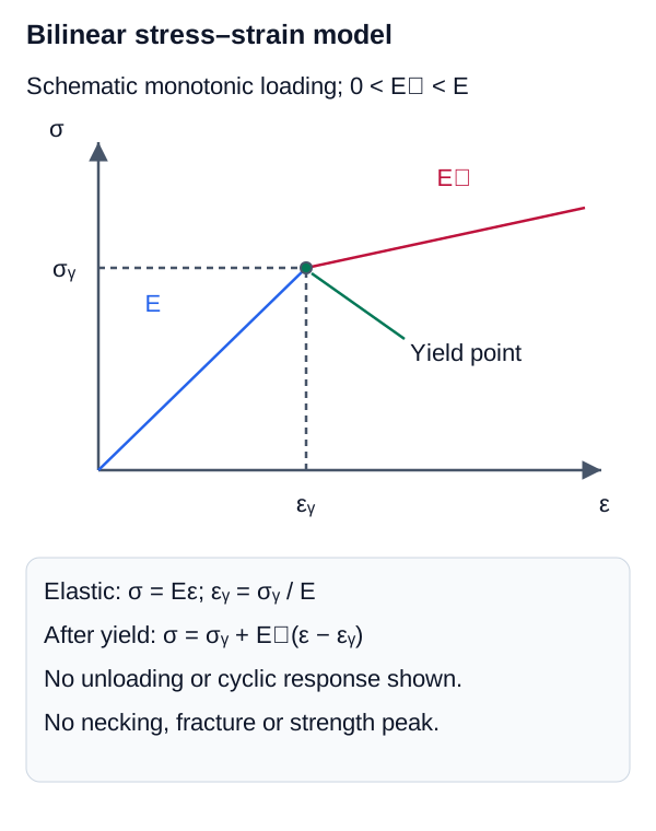
Constitutive definition

For σ ≤ σᵧ: ε = σ/E.

For σ > σᵧ: ε = εᵧ + (σ − σᵧ)/Eₜ.

In this deliberately simplified monotonic-loading law, the proportional limit and modeled yield point coincide. Real materials may not show that coincidence. Unloading and all ultimate/fracture behavior require a different constitutive model or material-specific data.

Normal stress σ

150.0 MPa

Strain ε

7.500e-4

Yield strain εᵧ

1.250e-3

Model state

LINEAR ELASTIC

Young's modulus E

200.00 GPa

Post-yield tangent Eₜ

4.00 GPa

Idealized bilinear stress-strain curve with linear elastic and strain-hardening branches — Explicit Bilinear Constitutive Model
The teaching model is linear elastic to its modeled yield point and then follows a lower tangent modulus. It does not represent ultimate strength, necking, or fracture.

$Scope of the Interactive Constitutive Model$

The interactive stress-strain curve is an explicitly idealized bilinear strain-hardening law. It is not a sourced material curve for steel, aluminum, titanium, copper, or any other specific alloy. In this idealization the proportional limit and modeled yield point coincide; real material data can distinguish these quantities and may exhibit nonlinear transition behavior.

$Types of Elastic Moduli$

The specific "Elastic Modulus" depends on the type of stress being applied. Common types include Young's Modulus, Shear Modulus, and Bulk Modulus.

$E$

Measures resistance to tension (stretching) or compression (squeezing) along one axis. This is crucial for designing columns and cables.

Young's Modulus Stress-Strain Equation

The fundamental relationship between stress and strain for tension or compression.

\sigma = E \epsilon

Variables

Symbol	Description	Unit
$\sigma$	Stress	Pa
$E$	Young's Modulus	Pa
$\epsilon$	Strain	dimensionless

Young's Modulus Force-Area Equation

Relates applied force, area, and length changes for tension or compression.

\frac{F}{A} = E \left(\frac{\Delta L}{L_0}\right)

Variables

Symbol	Description	Unit
$F$	Force applied	N
$A$	Cross-sectional area	$m^2$
$E$	Young's Modulus	Pa
$\Delta L$	Change in length	m
$L_0$	Original length	m

$G$

Measures resistance to shear forces (forces acting parallel to a surface, trying to slide layers past one another), where $\gamma$ is the shear strain angle.

Shear Modulus Equation

Hooke's Law applied to shear deformation.

\tau_{shear} = G \gamma

Variables

Symbol	Description	Unit
$\tau_{shear}$	Shear stress	Pa
$G$	Shear Modulus	Pa
$\gamma$	Shear strain	rad

$B$

Measures resistance to uniform compression from all sides (like an object submerged deep in the ocean). It relates pressure ( $P$ ) to volume strain ( $\Delta V/V_0$ ). The negative sign in the equation indicates that increased pressure causes a decrease in volume.

Bulk Modulus Equation

Relates pressure change to volume strain.

\Delta P = -B \left(\frac{\Delta V}{V_0}\right)

Variables

Symbol	Description	Unit
$\Delta P$	Change in pressure	Pa
$B$	Bulk Modulus	Pa
$\Delta V$	Change in volume	$m^3$
$V_0$	Original volume	$m^3$

Thermal Stress

$Thermal Stress Concepts$

If a structural member is constrained so that it cannot expand or contract when subjected to a temperature change ( $\Delta T$ ), large internal stresses develop. The thermal strain is $\epsilon_{thermal} = \alpha \Delta T$ . Because the member is constrained, the opposing stress developed is defined by the thermal stress equation.

Thermal Stress Equation

Calculates stress caused by constrained thermal expansion or contraction.

\sigma_{thermal} = E \alpha \Delta T

Variables

Symbol	Description	Unit
$\sigma_{thermal}$	Thermal stress	Pa
$E$	Young's Modulus	Pa
$\alpha$	Coefficient of linear expansion	$1/^\circ C$
$\Delta T$	Change in temperature	$^\circ C$

Normal, shear, volumetric, and restrained thermal deformation modes — Elastic Deformation Modes
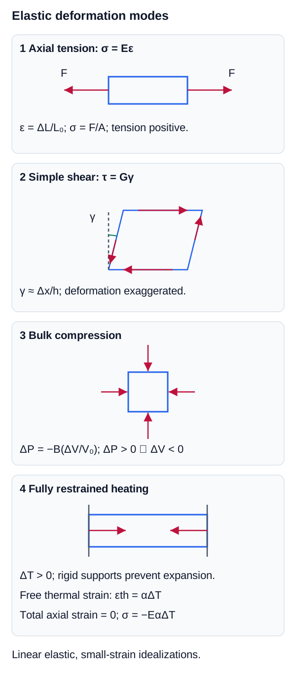
Young's, shear, and bulk moduli relate different conjugate stress-strain measures; thermal strain becomes stress only when expansion or contraction is restrained.

The Stress-Strain Curve

$The Stress-Strain Curve Concepts$

If you steadily increase the tensile stress on a material (like a steel rod) and plot the resulting strain, you get a characteristic curve.

$Landmarks on a Real Tensile Stress-Strain Curve$

Proportional limit: highest stress over which stress and strain remain proportional within the measurement/model definition.
Elastic limit: highest stress from which the material can unload without permanent strain; it is conceptually distinct from the proportional limit.
Yield: onset of appreciable plastic deformation, defined by a material-specific convention when a sharp yield point is absent.
Plastic region: deformation includes a permanent component after unloading.
Ultimate tensile strength: maximum engineering stress reached in a tensile test before the engineering-stress curve decreases during necking.
Fracture: specimen separation. It must not be inferred from a model that does not include a fracture criterion.

$Yield Strength Importance$

Engineering designs almost always require materials to stay well below their Yield Strength, ensuring they remain in the elastic region under typical operating loads.

Shear and Bulk Moduli

$Deformation Beyond Tension$

While Young's Modulus ( $E$ ) handles simple stretching and compression, complex structures experience other types of stress.

Shear Stress and Strain: Forces acting parallel to a surface cause layers of the material to slide past one another. The Shear Modulus ( $G$ ) relates shear stress ( $\tau = F_{parallel}/A$ ) to shear strain ( $\gamma = \Delta x / h$ ). This is critical in analyzing bolts, rivets, and torsion in drive shafts.
Bulk Stress and Strain: Forces acting uniformly from all directions (like hydrostatic pressure underwater) cause volume changes. The Bulk Modulus ( $B$ ) relates the change in pressure ( $\Delta P$ ) to the fractional change in volume ( $\Delta V / V_0$ ).

Shear Modulus Equation

Hooke's Law applied to shear deformation.

\tau = G \gamma

Variables

Symbol	Description	Unit
$\tau$	Shear stress	Pa
$G$	Shear Modulus	Pa
$\gamma$	Shear strain	rad

Key Takeaways

Static Equilibrium requires both zero net force ( $\Sigma \vec{F} = 0$ ) and zero net torque ( $\Sigma \vec{\tau} = 0$ ).
The Center of Gravity is the point where the total weight acts. It coincides with the center of mass for uniform fields.
Stress ( $\sigma = F/A$ ) measures the intensity of internal forces. Strain ( $\epsilon = \Delta L/L_0$ ) measures the resulting deformation.
Hooke's Law states that stress is proportional to strain in the elastic region, governed by an elastic modulus like Young's Modulus ( $E$ ).
The proportional limit, elastic limit, yield behavior, ultimate strength, and fracture are distinct material-response concepts; the interactive bilinear model represents only the elastic and post-yield branches stated in its constitutive definition.

$References$

Previous TopicRotational Motion - Theory & Concepts

Quiz Me

Next TopicFluid Mechanics - Theory & Concepts

Prev Next

Quiz Me

Learning Objectives

Static Equilibrium

Static Equilibrium Concepts

Translational Equilibrium Condition

Translational Equilibrium in 2D

Rotational Equilibrium Condition

Choosing an Axis of Rotation

Interactive Simulation

Center of Gravity (CG)

Center of Gravity (CG) Concepts

Center of Mass Location (xcmx_{cm}xcm​)

Center of Mass for Discrete Masses

Center of Mass for a Continuous Body

Elasticity and Deformation

Elasticity and Deformation Concepts

Stress (σ\sigmaσ)

Stress Equation

Strain (ϵ\epsilonϵ)

Strain Equation

Hooke's Law for Continua

Hooke's Law for Continua Concepts

Hooke's Law

Interactive Simulation

Scope of the Interactive Constitutive Model

Types of Elastic Moduli

Young's Modulus (EEE)

Young's Modulus Stress-Strain Equation

Young's Modulus Force-Area Equation

Shear Modulus (GGG)

Shear Modulus Equation

Bulk Modulus (BBB)

Bulk Modulus Equation

Thermal Stress

Thermal Stress Concepts

Thermal Stress Equation

The Stress-Strain Curve

The Stress-Strain Curve Concepts

Landmarks on a Real Tensile Stress-Strain Curve

Yield Strength Importance

Shear and Bulk Moduli

Deformation Beyond Tension

Shear Modulus Equation

References

$Learning Objectives$

$Static Equilibrium Concepts$

$Translational Equilibrium in 2D$

$Choosing an Axis of Rotation$

$Interactive Simulation$

$Center of Gravity (CG) Concepts$

$x_{cm}$

$Elasticity and Deformation Concepts$

$\sigma$

$\epsilon$

$Hooke's Law for Continua Concepts$

$Interactive Simulation$

$Scope of the Interactive Constitutive Model$

$Types of Elastic Moduli$

$E$

$G$

$B$

$Thermal Stress Concepts$

$The Stress-Strain Curve Concepts$

$Landmarks on a Real Tensile Stress-Strain Curve$

$Yield Strength Importance$

$Deformation Beyond Tension$

$References$