Oscillations and Waves
Learning Objectives
- Understand the principles of Simple Harmonic Motion (SHM) and compute related kinematics and energy.
- Analyze damped and driven oscillations and recognize the implications of resonance.
- Describe mechanical waves, wave properties, and their mathematical representations.
- Explain wave interference, the principle of superposition, and standing waves.
- Calculate the period of simple and physical pendulums.
- Understand sound waves and compute frequency shifts due to the Doppler Effect.
Oscillations and Simple Harmonic Motion (SHM)
Oscillations and Simple Harmonic Motion (SHM) Concepts
Motion that repeats after a fixed time interval is periodic. Harmonic motion is a more specific sinusoidal form of periodic motion; simple harmonic motion (SHM) occurs when the restoring acceleration is proportional to displacement and directed toward equilibrium.
Simple Harmonic Motion (SHM)
Motion caused by a restoring force that is directly proportional to the displacement from equilibrium and always directed towards that equilibrium position. This relationship is often described by Hooke's Law.
Hooke's Law for SHM
Relates the restoring force to the displacement from equilibrium.
Variables
| Symbol | Description | Unit |
|---|---|---|
| Restoring force | N | |
| Spring constant or stiffness | N/m | |
| Displacement from equilibrium | m |
Oscillations and Simple Harmonic Motion (SHM) Concepts
Because , the acceleration in SHM is also proportional to displacement: . This differential equation describes a system where the acceleration is always opposite to the position, leading to a sinusoidal oscillation.
Kinematics of SHM
Kinematics of SHM Concepts
The position (), velocity (), and acceleration () of an object in SHM as a function of time () are described by sinusoidal functions.
Position in SHM
Calculates the position of an object in SHM as a function of time.
Variables
| Symbol | Description | Unit |
|---|---|---|
| Position at time t | m | |
| Amplitude (maximum displacement) | m | |
| Angular frequency | rad/s | |
| Time | s | |
| Phase constant | rad |
Velocity in SHM
Calculates the velocity of an object in SHM as a function of time.
Variables
| Symbol | Description | Unit |
|---|---|---|
| Velocity at time t | m/s | |
| Amplitude | m | |
| Angular frequency | rad/s | |
| Time | s | |
| Phase constant | rad |
Acceleration in SHM
Calculates the acceleration of an object in SHM as a function of time.
Variables
| Symbol | Description | Unit |
|---|---|---|
| Acceleration at time t | ||
| Amplitude | m | |
| Angular frequency | rad/s | |
| Time | s | |
| Phase constant | rad | |
| Position at time t | m |
Angular Frequency Determinants
The angular frequency is determined entirely by the physical properties of the system (mass and stiffness), not by how the oscillation is started (amplitude).
Angular Frequency for a Mass-Spring System
Calculates the angular frequency for an ideal mass-spring system.
Variables
| Symbol | Description | Unit |
|---|---|---|
| Angular frequency | rad/s | |
| Spring constant | N/m | |
| Mass | kg |
Angular Frequency for a Simple Pendulum
Calculates the angular frequency for a simple pendulum at small angles.
Variables
| Symbol | Description | Unit |
|---|---|---|
| Angular frequency | rad/s | |
| Acceleration due to gravity | ||
| Length of the pendulum | m |
SHM Phase and Energy Exchange
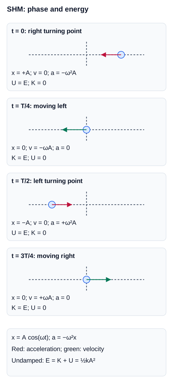
The deterministic phase sequence shows velocity peaking at equilibrium, acceleration opposing displacement, and kinetic and spring potential energy exchanging over one cycle.
Interactive Simulation
Switch between free and driven response. Vary mass, stiffness, damping ratio, driving force, and driving frequency to compare transient decay, steady-state amplitude, resonance, and phase lag.
Energy in SHM
Energy in SHM Concepts
In an ideal SHM system (no friction), the total mechanical energy () is conserved. Energy continuously transforms between kinetic and potential forms.
- Potential Energy (): Maximum at the extreme positions (), zero at equilibrium. .
- Kinetic Energy (): Maximum at equilibrium (), zero at the extremes. .
- Total Energy (): Constant. .
Damped and Driven Oscillations
Damped and Driven Oscillations Concepts
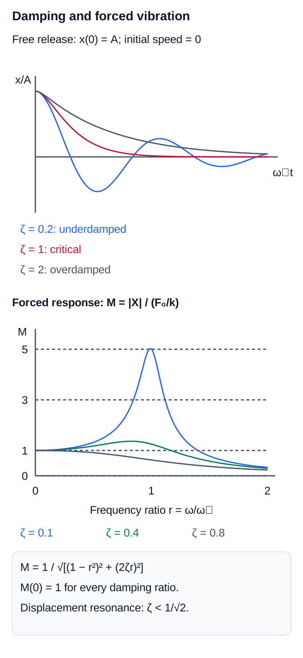
Real oscillators experience friction (damping), which removes energy and causes the amplitude to decay over time.
If an external periodic force is applied to the system, it is a driven oscillation. Every system has a natural frequency (). If the frequency of the driving force matches the natural frequency (), the amplitude of the oscillation can grow tremendously. This phenomenon is called Resonance.
Dynamic Amplification in Engineering
Resonance can produce large dynamic response when periodic excitation is near a system's natural frequency, especially when damping is low. Not every famous vibration failure is a simple resonance case: the 1940 Tacoma Narrows Bridge collapse is more accurately associated with aeroelastic instability rather than a textbook forced-resonance model.
Damping Regimes and Resonance Response
The time histories distinguish damping regimes, while the frequency-response panel shows how damping changes the height and breadth of the resonance peak.
Mechanical Waves
Mechanical Waves Concepts
While an oscillation is a local vibration, a wave is a disturbance that travels through a medium, transferring energy and momentum from point A to point B without transporting the matter of the medium itself.
Types of Waves
Types of Waves Concepts
- Transverse Waves: The particles of the medium oscillate perpendicular to the direction of wave propagation. Examples: Waves on a string, light (electromagnetic waves).
- Longitudinal Waves: The particles oscillate parallel to the direction of propagation (compressions and rarefactions). Examples: Sound waves in air or water, P-waves in earthquakes.
Wave Properties
Wave Properties Concepts
A periodic wave has a consistent shape that repeats in both space and time.
Wavelength ()
The spatial distance over which the wave shape repeats itself (e.g., crest to crest). The SI unit is meters (m).
Frequency ()
The number of complete wave cycles that pass a fixed point per unit time. The SI unit is Hertz (Hz), where .
Period ()
The time required for one complete cycle to pass a fixed point. Its SI unit is the second (s).
Period–Frequency Relationship
Relates period and frequency for periodic motion.
Variables
| Symbol | Description | Unit |
|---|---|---|
| Period | s | |
| Frequency | Hz |
Wave Speed Equation
Calculates the speed at which the wave disturbance propagates through the medium.
Variables
| Symbol | Description | Unit |
|---|---|---|
| Wave speed | m/s | |
| Frequency | Hz | |
| Wavelength | m | |
| Period | s |
Wave Speed Determinants
For a specified wave mode in an ideal nondispersive medium, propagation speed is set by the medium's constitutive and inertial properties rather than by amplitude. For sound in an ideal gas of fixed composition, speed depends primarily on absolute temperature; real media can also be dispersive, so phase or group speed may vary with frequency.
The Mathematical Description of a Wave
The Mathematical Description of a Wave Concepts
A 1D harmonic wave traveling in the positive x-direction can be described by a wave function , which gives the transverse displacement of a particle at position and time .
Wave Function
Describes the transverse displacement of a particle at position x and time t for a 1D harmonic wave.
Variables
| Symbol | Description | Unit |
|---|---|---|
| Transverse displacement at position x and time t | m | |
| Amplitude | m | |
| Wave number (2\pi / \lambda) | rad/m | |
| Position | m | |
| Angular frequency (2\pi f) | rad/s | |
| Time | s |
Traveling and Standing Waves
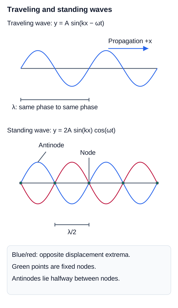
The upper trace identifies wavelength and travel direction; the lower trace identifies the stationary node and antinode pattern produced by counter-propagating waves.
Energy and Intensity of Waves
Energy and Intensity of Waves Concepts
Waves transport energy. The power () transmitted by a harmonic wave on a string is proportional to the square of its amplitude and the square of its frequency.
For 3D waves (like sound or light), we describe the energy flow using Intensity (), which is the power transmitted across a unit area perpendicular to the direction of propagation.
Wave Intensity
Calculates the energy flow per unit area for 3D waves like sound or light.
Variables
| Symbol | Description | Unit |
|---|---|---|
| Intensity | ||
| Power transmitted by the wave | W | |
| Area perpendicular to the direction of wave propagation |
Energy and Intensity of Waves Concepts
For a point source emitting energy equally in all directions (spherical waves), the intensity decreases as the inverse square of the distance () from the source: .
Interference and Standing Waves
Interference and Standing Waves Concepts
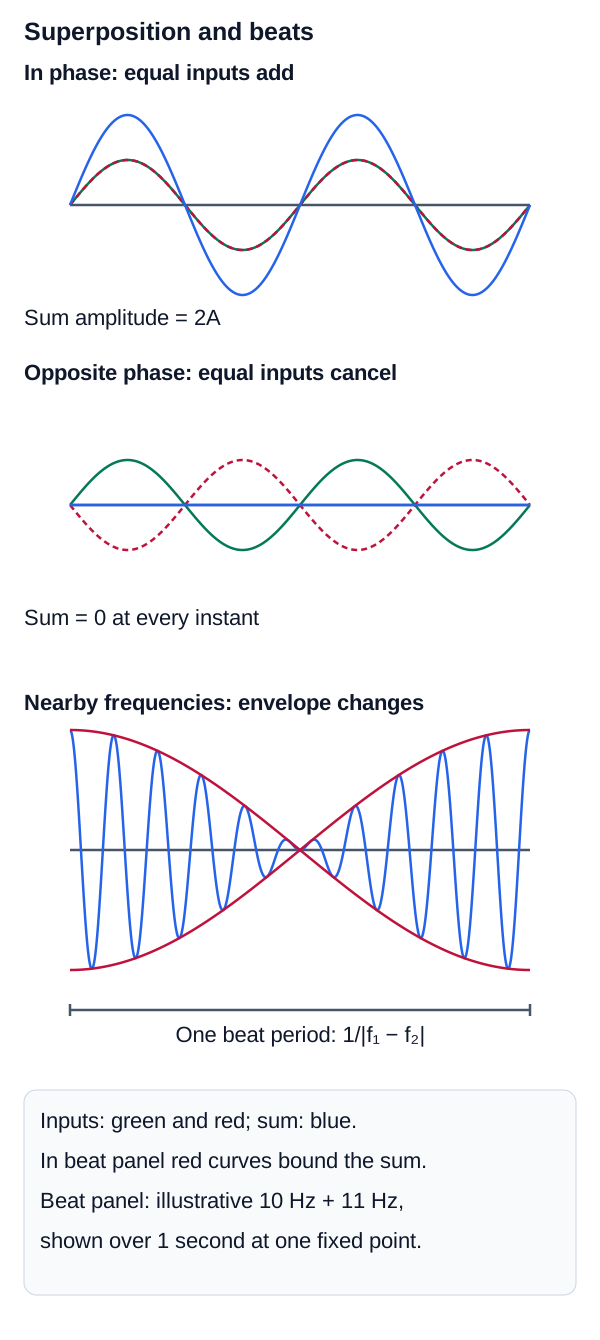
When two or more waves travel through the same medium simultaneously, they obey the Principle of Superposition: The net displacement of the medium at any point is the algebraic sum of the individual wave displacements at that point.
- Constructive Interference: Waves arrive "in phase" (crest meets crest), resulting in a larger combined amplitude.
- Destructive Interference: Waves arrive "out of phase" (crest meets trough), resulting in a smaller or zero combined amplitude.
When two identical waves traveling in opposite directions interfere, they create a Standing Wave. The wave appears to vibrate in place rather than travel.
Nodes and Antinodes
- Nodes: Points on a standing wave that never move (complete destructive interference).
- Antinodes: Points that oscillate with maximum amplitude (constructive interference).
Interference and Standing Waves Concepts
Two coherent waves of the same frequency traveling in opposite directions can form a standing-wave pattern. In a bounded system such as a string fixed at both ends, the boundary conditions permit only discrete normal-mode frequencies; these resonant frequencies form the allowed harmonics.
Interference and Temporal Beats
The superposition panels distinguish phase-controlled interference from beats, whose envelope repeats at the actual temporal frequency difference |fA-fB|.
Interactive Simulation
Keep the propagation speed fixed while changing frequency to see wavelength respond through v=fλ. The time probe uses each wave's own angular frequency, so nearby frequencies generate a real temporal beat envelope at |fA-fB|.
The Simple and Physical Pendulum
Pendulum Mechanics
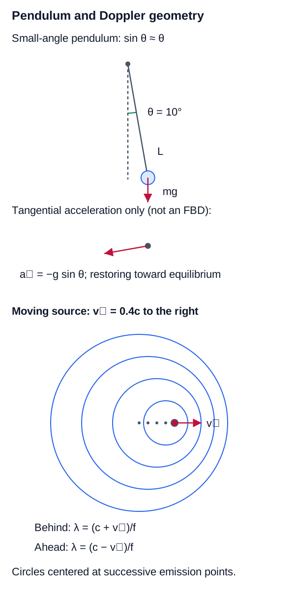
A Simple Pendulum consists of a point mass () suspended by a massless, unstretchable string of length . For sufficiently small angular displacements, (with in radians), so the restoring torque is approximately proportional to angular displacement and the pendulum behaves as SHM. The approximation becomes progressively less accurate as amplitude increases.
A Physical Pendulum is any real, rigid object swinging from a pivot point. Its period depends on its Moment of Inertia () about the pivot and the distance () from the pivot to its center of gravity.
Period of a Physical Pendulum
Calculates the time required for one complete swing of a rigid body pendulum.
Variables
| Symbol | Description | Unit |
|---|---|---|
| Period | s | |
| Moment of Inertia about pivot | ||
| Mass | kg | |
| Distance from pivot to center of mass | m |
Pendulum Geometry and Doppler Wavefronts
The pendulum panel identifies the small-angle restoring geometry; the Doppler panel shows shorter wavefront spacing ahead of a moving source and longer spacing behind it.
Sound Waves and the Doppler Effect
The Doppler Effect
Sound waves are longitudinal mechanical waves. When a source of sound and an observer are in relative motion, the observer perceives a frequency different from the one emitted by the source. This is the Doppler Effect.
If the source and observer are moving towards each other, the perceived frequency increases (higher pitch). If they are moving apart, the perceived frequency decreases.
The Doppler Effect Equation
Calculates the observed frequency of a wave due to relative motion.
Variables
| Symbol | Description | Unit |
|---|---|---|
| Observed frequency | Hz | |
| Source frequency | Hz | |
| Speed of sound in the medium | m/s | |
| Speed of the observer | m/s | |
| Speed of the source | m/s |
Doppler Sign Convention
Choose the observer sign so motion toward the source increases the numerator, and choose the source sign so motion toward the observer decreases the denominator. A velocity diagram is safer than memorizing signs when both source and observer move.
- Simple Harmonic Motion (SHM) occurs when a restoring force is proportional to displacement (). It is described by sinusoidal functions ().
- The angular frequency () of SHM depends on the system's mass and stiffness, not amplitude. Resonance occurs when a driving frequency matches this natural frequency.
- Waves transfer energy through a medium. They are characterized by wavelength (), frequency (), and wave speed (). For a given nondispersive wave mode, wave speed is set by the medium rather than by source amplitude.
- Transverse waves oscillate perpendicular to propagation; Longitudinal waves oscillate parallel.
- Interference (superposition) leads to phenomena like Standing Waves, characterized by nodes (zero amplitude) and antinodes (max amplitude).