Deflection of Structures - Theory & Concepts

Deflection of Structures - Theory & Concepts

$Learning Objectives$

Understand the fundamental principles governing beam deflection.
Apply geometric methods such as the Double Integration Method, Moment-Area Method, and Conjugate Beam Method.
Apply energy methods including Virtual Work (Unit Load Method) and Castigliano's Theorems.
Understand and apply Maxwell-Betti's Reciprocal Theorem.

Deflection is the displacement of a structural element under load. Controlling deflection is critical for ensuring the serviceability (usability and comfort) of a structure, preventing damage to non-structural elements (partitions, ceilings), and ensuring visual acceptability.

Fundamental Principles

The relationship between load, shear, moment, slope, and deflection is governed by differential equations derived from beam theory.

Beam Deflection Relationships

The fundamental differential equations relating load, shear, moment, slope, and deflection.

E I \frac{d^4v}{dx^4} = -w(x)

E I \frac{d^3v}{dx^3} = V(x)

E I \frac{d^2v}{dx^2} = M(x)

\frac{dv}{dx} = \theta(x)

Variables

Symbol	Description	Unit
$E$	Modulus of Elasticity	-
$I$	Moment of Inertia	-
$E I$	Flexural Rigidity	-
$v(x)$	Deflection	-
$w(x)$	Load	-
$V(x)$	Shear	-
$M(x)$	Moment	-
$\theta(x)$	Slope	-

$Interactive Simulation$

Explore how load, length, and material properties affect beam deflection with this interactive tool:

Geometric Methods

These methods rely on the geometry of the elastic curve (deflected shape).

The Double Integration Method

The Double Integration Method involves solving the governing differential equation for the elastic curve of a beam to find expressions for its slope and deflection everywhere along its length.

$Integration Process$

Sign Convention: A positive internal moment $M(x)$ causes the beam to bend concave upwards (like a smile). In this standard coordinate system, a positive deflection $v$ indicates an upward displacement, and a negative deflection indicates a downward displacement.

First Integration: Integrating the equation once yields the equation for the slope ( $\theta$ ) of the elastic curve, plus a constant of integration ( $C_1$ ).
Second Integration: Integrating a second time yields the equation for the deflection ( $v$ ), plus another constant ( $C_2$ ).
Boundary Conditions: To solve for the constants $C_1$ and $C_2$ , the known geometric boundary conditions of the beam's supports are applied (e.g., at a fixed support, deflection $v=0$ and slope $\theta=0$ ; at a pin or roller, deflection $v=0$ ).

Governing Differential Equation

The foundational relationship between bending moment and deflection derived from beam theory.

E I \frac{d^2 v}{d x^2} = M(x)

Variables

Symbol	Description	Unit
$E$	Modulus of elasticity	-
$I$	Moment of inertia	-
$v$	Vertical deflection	-
$x$	Position along the beam	-
$M(x)$	Internal bending moment expressed as a function of $x$	-

First Integration (Slope)

Equation for the slope of the elastic curve.

E I \frac{d v}{d x} = \int M(x) dx + C_1

Variables

Symbol	Description	Unit
$C_1$	First constant of integration	-

Second Integration (Deflection)

Equation for the deflection of the elastic curve.

E I v = \iint M(x) dx dx + C_1 x + C_2

Variables

Symbol	Description	Unit
$C_2$	Second constant of integration	-

Macaulay's Method (Singularity Functions)

For beams with multiple loads, the internal moment $M(x)$ changes equations at every load point. Macaulay's Method uses singularity functions (Macaulay brackets, e.g., $\langle x - a \rangle$ ) to write a single, continuous equation for $M(x)$ valid across the entire beam length. This reduces the number of integration constants from $2n$ (where $n$ is the number of beam segments) down to just 2 for the whole beam, drastically simplifying the double integration process.

Moment-Area Method

Based on two theorems relating the area of the $M/EI$ diagram to changes in slope and deflection.

$First Moment-Area Theorem$

The change in slope between any two points on the elastic curve equals the area of the $M/EI$ diagram between those points.

First Moment-Area Theorem Equation

Change in slope between points A and B.

\Delta \theta_{AB} = \int_A^B \frac{M}{EI} dx

Variables

Symbol	Description	Unit
$\Delta \theta_{AB}$	Change in slope between point A and point B	-
$M$	Internal bending moment	-
$E$	Modulus of elasticity	-
$I$	Moment of inertia	-

$Second Moment-Area Theorem$

The vertical deviation of point B on the elastic curve from the tangent drawn at point A equals the moment of the area of the $M/EI$ diagram between A and B, taken about B.

Second Moment-Area Theorem Equation

Vertical deviation of point B from tangent drawn at point A.

t_{B/A} = \int_A^B \frac{M}{EI} x dx

Variables

Symbol	Description	Unit
$t_{B/A}$	Vertical deviation of B with respect to the tangent at A	-
$M$	Internal bending moment	-
$E$	Modulus of elasticity	-
$I$	Moment of inertia	-
$x$	Distance from the moment center (point B)	-

Conjugate Beam Method

Transforms the real beam into a fictitious "conjugate beam" loaded with the $M/EI$ diagram of the real beam.

$Conjugate Beam Correspondences$

STEP-BY-STEP

Slope on real beam $\leftrightarrow$ Shear on conjugate beam.
Deflection on real beam $\leftrightarrow$ Moment on conjugate beam.

$Interactive Simulation$

Use this interactive tool to explore the Conjugate Beam Method:

Adjust the load position to see how the M/EI diagram becomes the load for the Conjugate Beam.

Real Beam (Point Load)

Conjugate Beam (M/EI Load)

Energy Methods

Based on the principle of conservation of energy (Work Done = Strain Energy Stored). These are incredibly versatile methods applicable to all structural types.

Virtual Work (Unit Load Method)

A powerful and versatile method applicable to beams, frames, and trusses.

$Virtual Work Procedure$

STEP-BY-STEP

To find deflection at a point, apply a virtual unit load at that point in the direction of the desired displacement.
Calculate internal virtual forces ( $m$ ) due to the unit load, and calculate real internal forces ( $M$ ) due to actual loads.

Virtual Work Equation (Beams)

Calculates deflection using virtual work.

1 \cdot \Delta = \int_0^L \frac{M m}{EI} dx

Variables

Symbol	Description	Unit
$\Delta$	Deflection	-
$M$	Real moment function	-
$m$	Virtual moment function due to unit load	-
$E$	Modulus of elasticity	-
$I$	Moment of inertia	-

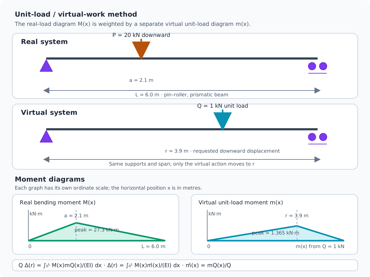
Simply supported beam with a real point load, a separate one-kilonewton unit load, and their M(x) and m(x) moment diagrams for the unit-load method. — Unit-load method: real and virtual moment diagrams
The real-load moment diagram M(x) and the virtual unit-load diagram m(x) are multiplied and integrated over EI to obtain the displacement at response location r. The physical beam sketches use a six-metre span; the graphs are explicitly separate, independently scaled plots.

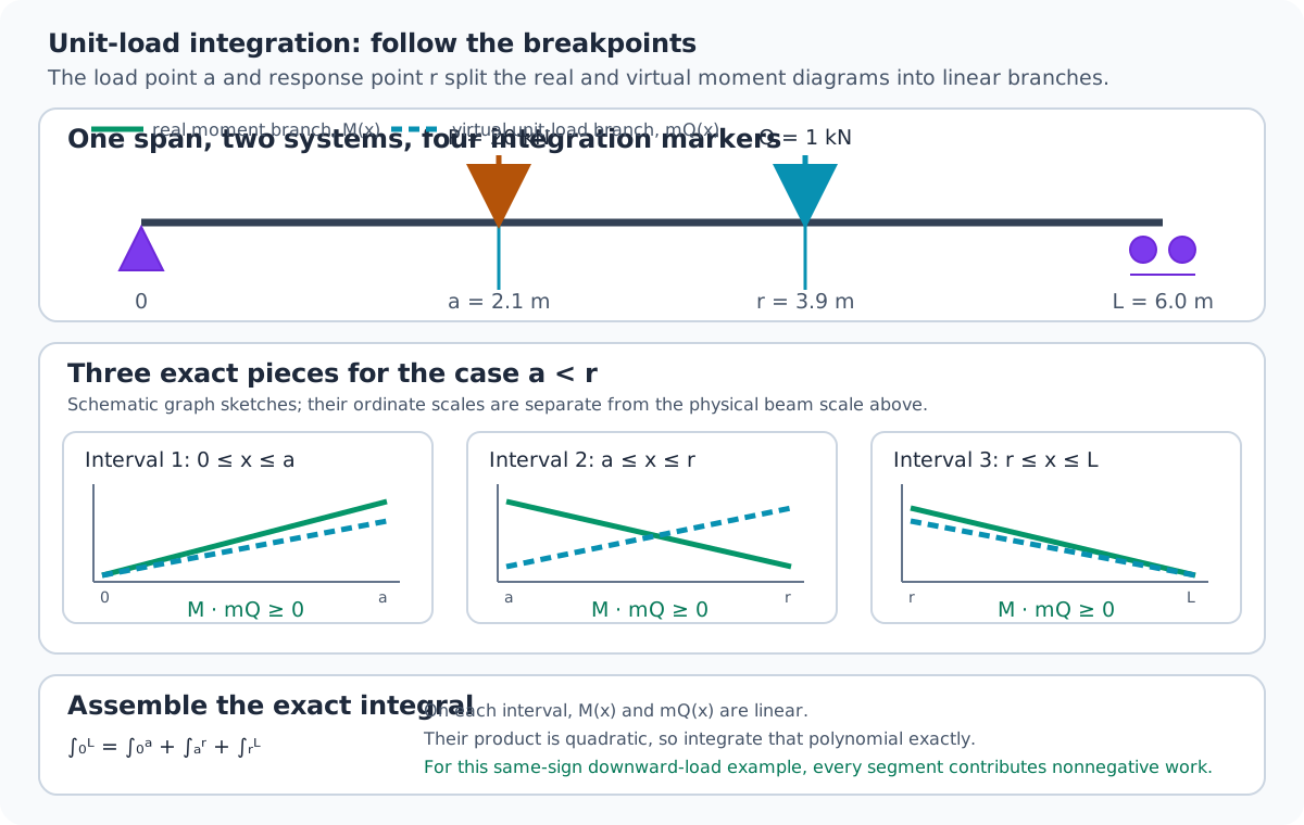
Piecewise unit-load integration map showing the real-load moment, virtual unit-load moment, load point a, response point r, and the three integration intervals from zero to a, a to r, and r to L. — Piecewise integration segments for the unit-load method
For the illustrative case where the real load point a lies left of response point r, the four span markers divide the diagrams into three intervals. On each interval the real and virtual moment branches are linear, so their product is integrated exactly as a quadratic polynomial.

$Interactive Unit-Load Deflection Simulation$

Use the simulation to move the real point load and the response location independently. Read how the exact piecewise integral of $M(x)m(x)/(EI)$ changes when the virtual unit load moves, while $E$ and $I$ control flexural rigidity.

Beam and material controls

Point load20 kN

Span6.0 m

Real load position as span fraction0.35

Response location as span fraction0.65

Elastic modulus200 GPa

Moment of inertia200 ×10⁶ mm⁴

Actual positions:

a

= 2.10 m and

r

= 3.90 m. The virtual action is

Q = 1\ \mathrm{kN}

Q\Delta(r) = \int_0^L \frac{M(x)m_Q(x)}{EI}\,dx

The virtual bending-moment diagram is generated by the one-kilonewton action at the response location. The reported displacement divides the internal virtual work by that action.

Exact integration method

On each of 3 intervals, $M(x)$ and $m_Q(x)$ are linear. Their product is integrated as a quadratic polynomial; the only numerical limitation is floating-point round-off.

Real-load moment diagram; peak = 27.30 kN·m.

Virtual unit-load moment diagram; peak = 1.36 kN·m.

Displacement at response location

1.665 mm downward

The reported displacement equals internal virtual work divided by the one-kilonewton virtual action.

Flexural rigidity

4.000e+4 kN·m²

The converted modulus and section inertia are multiplied to form flexural rigidity.

Virtual work before division

1.665e-3 kN·m

Internal virtual work evaluated from the exact piecewise integral.

Response position

3.90 m

The real point load is at 2.10 m.

\Delta(r) = \int_0^L \frac{M(x)\,\bar m(x)}{EI}\,dx

The normalized form uses $\bar m(x) = m_Q(x)/Q$ . Moving the response location changes only the virtual diagram, so its overlap with the real diagram explains the change in displacement.

Castigliano's Theorems

Alberto Castigliano formulated two essential theorems using partial derivatives of strain energy to find displacements and forces.

$Castigliano's First Theorem Context$

For a linearly elastic structure, the partial derivative of the total strain energy ( $U$ ) with respect to a specific displacement ( $\Delta_i$ ) gives the applied force ( $P_i$ ) corresponding to that displacement.

Note: This theorem is primarily used in advanced structural mechanics to formulate stiffness matrices.

Castigliano's First Theorem

Finds applied force from strain energy.

P_i = \frac{\partial U}{\partial \Delta_i}

Variables

Symbol	Description	Unit
$P_i$	Applied force	-
$U$	Total strain energy	-
$\Delta_i$	Displacement at point of application	-

$Castigliano's Second Theorem Context$

For a linearly elastic structure, the partial derivative of the total strain energy ( $U$ ) with respect to an applied force ( $P_i$ ) is equal to the displacement ( $\Delta_i$ ) at the point of application and in the specific direction of that force.

Note: This is the theorem most frequently used by engineers to calculate deflections. For example, for a beam subject to bending, $U = \int \frac{M^2}{2EI} dx$ , thus $\Delta = \int \frac{M}{EI} \frac{\partial M}{\partial P} dx$ .

Castigliano's Second Theorem

Finds displacement from strain energy.

\Delta_i = \frac{\partial U}{\partial P_i}

Variables

Symbol	Description	Unit
$\Delta_i$	Displacement at point of application	-
$U$	Total strain energy	-
$P_i$	Applied force	-

Maxwell-Betti's Reciprocal Theorem

The reciprocal theorem establishes a profound symmetry in linear elastic structures.

$Betti's Law$

A general theorem which states that the virtual work done by a first set of forces ( $P_i$ ) moving through the actual displacements caused by a second set of forces ( $P_j$ ) is equal to the virtual work done by the second set of forces ( $P_j$ ) moving through the actual displacements caused by the first set of forces ( $P_i$ ).

Betti's Law Equation

Equality of virtual work done by reciprocal forces.

\sum P_i \Delta_{ij} = \sum P_j \Delta_{ji}

Variables

Symbol	Description	Unit
$P_i$	First set of forces	-
$\Delta_{ij}$	Actual displacements caused by second set of forces	-
$P_j$	Second set of forces	-
$\Delta_{ji}$	Actual displacements caused by first set of forces	-

$Maxwell's Reciprocal Theorem$

A special, simplified case of Betti's Law where both sets of forces are single unit loads ( $P_i = 1$ , $P_j = 1$ ). It states that the displacement at point A due to a unit load applied at point B is exactly equal to the displacement at point B due to a unit load applied at point A.

For linear-elastic conservative reciprocal structural systems under the usual stiffness-method assumptions, the stiffness matrix ( $[K]$ ) and corresponding flexibility matrix ( $[F]$ , when it exists) are symmetric about the main diagonal.

Maxwell's Reciprocal Theorem Equation

Reciprocal displacement for unit loads.

\delta_{AB} = \delta_{BA}

Variables

Symbol	Description	Unit
$\delta_{AB}$	Displacement at A due to unit load at B	-
$\delta_{BA}$	Displacement at B due to unit load at A	-

Key Takeaways

Deflection ( $v$ ) is a crucial check for serviceability limit states, ensuring structures remain functional and undamaged under regular use.
The governing differential equations form the basis of calculation methods like double integration. The sign convention (usually $v$ positive upwards) must be strictly maintained.
Moment-Area Method uses geometric properties of the $M/EI$ diagram (best for prismatic beams with simple loadings).
Conjugate Beam Method simplifies deflection calculations by transforming them into basic statics problems (finding internal moment on a fictitious beam).
Energy Methods leverage the principle of conservation of energy to determine deflections efficiently, especially for complex geometries like trusses and frames.
Virtual Work (Unit Load) is the most versatile deflection method.
Castigliano's Second Theorem calculates displacements directly by taking the partial derivative of the strain energy equation with respect to an applied point load.

Previous TopicInfluence Lines for Determinate Structures - Examples & Applications

Quiz Me

Next TopicDeflection of Structures - Examples & Applications

Prev Next

Quiz Me